Addendum to Data Visualization posts #21 and #22

In data visualization posts #21 and #22, I referred to the results of simple multivariate linear regressions where I examined the statistical relationships between the cost of electricity across European Union countries and the market penetration of renewable energy sources, and a cost-of-living index. Here are the regression results that form the source data for the predictive plots in those blog posts.

First, with the price of electricity as the dependent variable (DV):

## Here is the R code for the linear regression (using the generalized linear models (glm) framework:
glm.1<-glm(Elec_Price~COL_Index+Pct_Share_Total,data=eu.RENEW.only,family="gaussian")  # Electricity Price is DV


MODEL INFO:
Observations: 28
Dependent Variable: Price of Household Electricity (in Euro cents)
Type: Linear regression 

MODEL FIT:
χ²(2) = 306.82, p = 0.00
Pseudo-R² (Cragg-Uhler) = 0.40
Pseudo-R² (McFadden) = 0.08
AIC = 166.04, BIC = 171.37 

Standard errors: MLE
-------------------------------------------------------------
                                 Est.   S.E.   t val.      p
------------------------------ ------ ------ -------- ------
(Intercept)                     4.10   3.59     1.14   0.26
Cost-of-Living Index            0.22   0.06     3.59   0.00
Renewables (% share of total)   0.03   0.04     0.74   0.46
-------------------------------------------------------------

We can see that the cost-of-living index is positively correlated with the price of household electricity, and it is statistically significant at conventional (p=0.05) levels. The market penetration of renewables (on the other hand) is not statistically significant (once controlling for cost-of-living.

Now, we use the pre-tax price of electricity (there are large differences in levels of taxation of household electricity across EU countries) as the DV. Here are the regression code (R) and the model results of the multivariate linear regression.

## Here is the R code for the linear regression (using the generalized linear models (glm) framework:

glm.2<-glm(Elec_Price_NoTax~COL_Index+Pct_Share_Total,data=eu.RENEW.only,family="gaussian")  # Elec Price LESS taxes/levies is DV


MODEL INFO:
Observations: 28
Dependent Variable: Pre-tax price of Household Electricity (Euro cents)
Type: Linear regression 

MODEL FIT:
χ²(2) = 100.13, p = 0.00
Pseudo-R² (Cragg-Uhler) = 0.44
Pseudo-R² (McFadden) = 0.12
AIC = 130.11, BIC = 135.43 

Standard errors: MLE
-------------------------------------------------------------
                                 Est.   S.E.   t val.      p
-----------------------------  ------- ------ -------- ------
(Intercept)                      5.20   1.89     2.75   0.01
Cost-of-Living Index             0.14   0.03     4.41   0.00
Renewables (% share of total)   -0.03   0.02    -1.44   0.16
-------------------------------------------------------------

Here, we see an even stronger relationship between the cost-of-living and the pre-tax price of household electricity, while there is (once the cost-of-living is controlled for) a negative (though not quite statistically significant) relationship between the pre-tax cost of electricity and the market penetration of renewables across EU countries.

Data Visualization #22—EU Electricity Prices (Part II)

In post #21 of this series, I examined the relationship between electricity prices across European Union (EU) countries and the market penetration of renewable (solar and wind) energy sources. There’s been some discussion amongst the defenders of the continued uninterrupted burning of fossil fuels of a finding that allegedly shows the higher the market penetration of renewables, the higher electricity prices. I demonstrated in the previous post that this is a spurious relationship and a more plausible reason for the empirical relationship is that market penetration is highly correlated with how rich (and expensive) a country is. Indeed, I showed that controlling for cost-of-living in a particular country, the relationship between market penetration of renewables and cost of electricity was not statistically significant.

I noted at the end of that post that I would show the results of a simple multiple linear regression of the before-tax price of electricity and market penetration of renewables across these countries.

But, first here is a chart of the results of the predicted price of before-tax electricity in a country given the cost-of-living, holding the market penetration of renewables constant. We see a strong positive relationship—the higher the cost-of-living in a country, the more expensive the before-tax cost of electricity.

Created by: Josip Dasović

Here’s the chart based on the results of a multiple regression analysis using before-tax electricity price as the dependent variable, with renewables market penetration as the main dependent variable, holding the cost-of-living constant. The relationship is obviously negative, but it is not statistically significant. Still, there is NOT a positive relationship between the market penetration of renewables and the before-tax price of electricity across EU countries.

Created by: Josip Dasović

How to lie with Statistics

In class last week, we were introduced to recent research on the effect of same-sex parenting on children’s welfare, specifically on high school graduation rates. We discussed how easy it can be to manipulate data in order to present a distorted view of reality.

I’ll use a fictitious example to make the point. Let’s assume you had two schools–Sir Charles Tupper and William Gladstone. Assume further that the graduation rates of the two schools are 98% and 94% for Tupper and Gladstone, respectively. Is one school substantially better at graduating its students than the other? Not really. In fact, the graduation rate at Tupper is about 4.3% higher than at Gladstone. So, Tupper is marginally better at graduating students than is Gladstone.

But, what if we compared non-graduation rates instead? Well, the non-graduation rate at Tupper is 2%, while the non-graduation rate at Gladstone is 6%. Thus, the following accurate statistical claim can legitimately be made: “Gladstone’s drop-out [non-graduation] rate is 300% greater than is Tupper’s.” Or, “Tupper non-graduation rate is 33% of Gladstone’s!” Would parents’ reactions be the same if the data were presented in this manner?

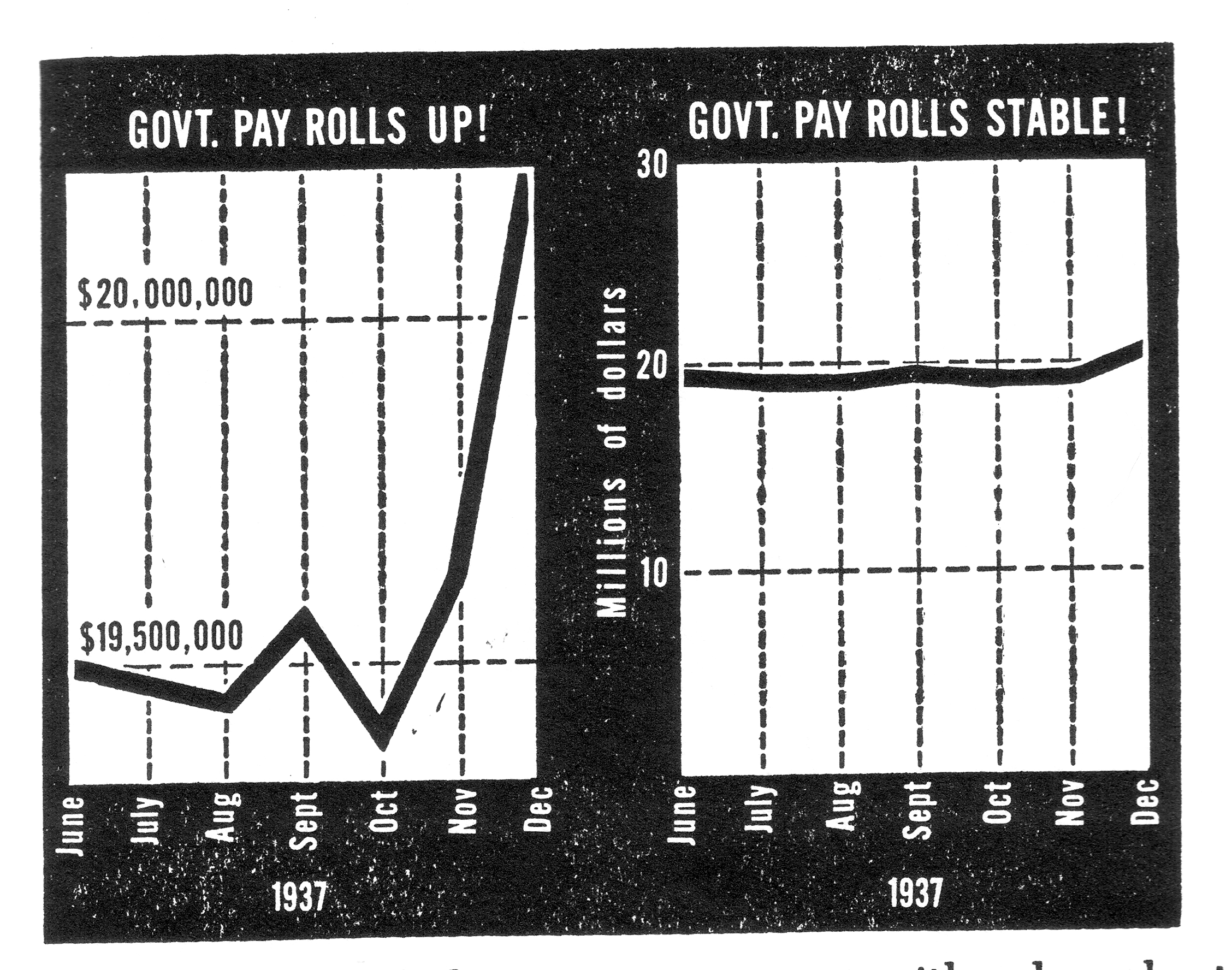
Another way to lie with statistics using graphs.

A new Measure of State Capacity

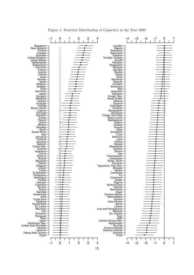
In a recent working paper by Hanson and Sigman, of the Maxwell School of Citizenship and Public Affairs at Syracuse University, the authors explore the concept(s) of state capacity. The paper title–Leviathan’s Latent Dimensions: Measuring State Capacity for Comparative Political Research, complies with my tongue-in-cheek rule about the names of social scientific papers. Hanson and Sigman use statistical methods (specifically, latent variable analysis) to tease out the important dimensions of state capacity. Using a series of indexes created by a variety of scholars, organizations, and think tanks, the authors conclude that there are three distinct dimensions of state capacity, which they label i) extractive, ii) coercive, and iii) administrative state capacity.

Here is an excerpt:

The meaning of state capacity varies considerably across political science research. Further complications arise from an abundance of terms that refer to closely related attributes of states: state strength or power, state fragility or failure, infrastructural power, institutional capacity, political capacity, quality of government or governance, and the rule of law. In practice, even when there is clear distinction at the conceptual level, data limitations frequently lead researchers to use the same
empirical measures for differing concepts.

For both theoretical and practical reasons we argue that a minimalist approach to capture the essence of the concept is the most effective way to define and measure state capacity for use in a wide range of research. As a starting point, we define state capacity broadly as the ability of state institutions to effectively implement official goals (Sikkink, 1991). This definition avoids normative conceptions about what the state ought to do or how it ought to do it. Instead, we adhere to the notion that capable states may regulate economic and social life in different ways, and may achieve these goals through varying relationships with social groups…

…We thus concentrate on three dimensions of state capacity that are minimally necessary to carry out the functions of contemporary states: extractive capacity, coercive capacity, and administrative capacity. These three dimensions, described in more detail below,accord with what Skocpol identifies as providing the “general underpinnings of state capacities” (1985: 16): plentiful resources, administrative-military control of a territory, and loyal and skilled officials.

Here is a chart that measures a slew of countries on the extractive capacity dimension in extractive_capacity

Indicators and The Failed States Index

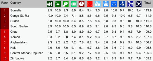
The Failed State Index is created and updated by the Fund for Peace. For the most recent year (2013), the Index finds the same cast of “failed” characters as previous years. There is some movement, the “top” 10 has not changed much over the last few years.

The Top 10 of the Failed States Index for 2013

Notice the columns in the image above. Each of these columns is a different indicator of “state-failedness”. If you go to the link above, you can hover over each of the thumbnails to find out what each indicator measures. For, example, the column with what looks like a 3-member family is the score for “Mounting Demographic Pressures”, etc. What is most interesting about the individual indicator scores is how similar they are for each state. In other words, if you know Country X’s score on Mounting Demographic Pressures, you would be able to predict the scores of the other 11 indicators with high accuracy. How high? We’ll just run a simple regression analysis, which we’ll do in IS240 later this semester.

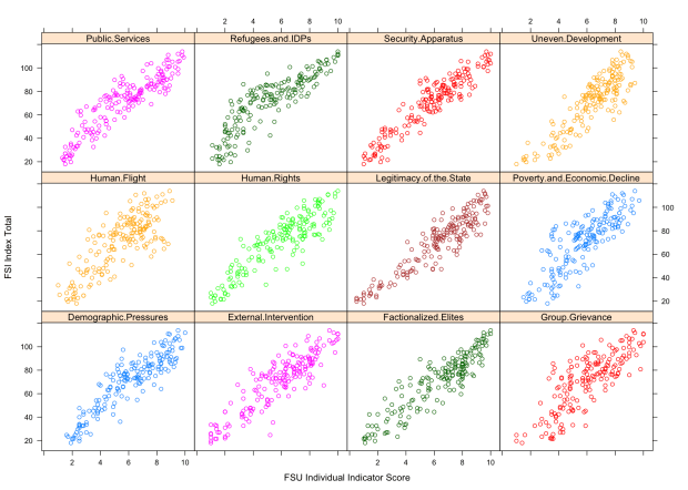
For now, though, I was curious as to how closely each indicator was correlated with the total score. Rather than run regression analyses, I chose (for now) to simply plot the associations. [To be fair, one would want to plot each indicator not against the total but against the total less that indicator, since each indicator comprises a portion (1/12, I suppose) of the total score. In the end, the general results are similar,if not exactly the same.]

So, what does this look like? See the image below (the R code is provided below, for those of you in IS240 who would like to replicate this.)

Plotting each of the Failed State Index (FSI) Indicators against the Total FSI Score

Here are two questions that you should ponder:

  1. If you didn’t have the resources and had to choose only one indicator as a measure of “failed-stateness”, which indicator would you choose? Which would you definitely not choose?
  2. Would you go to the trouble and expense of collecting all of these indicators? Why or why not?

R-code:


install.packages("gdata") #This package must be installed to import .xls file

library(gdata) #If you find error message--"required package missing", it means that you must install the dependent package as well, using the same procedure.

fsi.df<-read.xls("http://ffp.statesindex.org/library/cfsis1301-fsi-spreadsheet178-public-06a.xls")  #importing the data into R, and creating a data frame named fsi.df

pstack.1<-stack(fsi.df[4:15]) #Stacking the indicator variables in a single variable

pstack.df<-data.frame(fsi.df[3],pstack.1) #setting up the data correctly

names(pstack.df)<-c("Total","Score","Indicator") #Changing names of Variables for presentation

install.packages("lattice")  #to be able to create lattice plots

library(lattice) #to load the lattice package

xyplot(pstack.df$Total~pstack.df$Score|pstack.df$Indicator,  groups=pstack.df$Indicator, layout=c(4,3),xlab="FSI Individual Indicator Score", ylab="FSI Index Total")

Where do most of the World’s Poor Live?

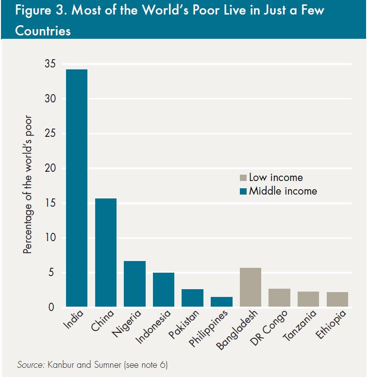
In a recently released report. the Center for Global Development argues that there are more poor people in middle-income countries (MICs) than in low-income countries (LICs). The new “bottom billion” (the phrase made famous by economic Paul Collier’s book of the same name) is not only the result of India and China having moved from LIC to MIC status. Indeed, according to the authors of the report, “the proportion of the world’s poor in MICs has still tripled, not only from a range of other countries like Nigeria, Pakistan, Indonesia, but also from some surprising MIC countries such as Sudan, Angola, and Cameroon.” Whereas twenty years ago, more than 90% of the world’s poor lived in LICs, today more than 70% of the world’s poor live in MICs.

Since 2000, over 700 million poor people have “moved” into MICs by way of their countries’ graduating from low-income status (see figure 1). And this is not just about China and India. Even without them, the proportion of the world’s poor in MICs has still tripled, not only from a range of other countries like Nigeria, Pakistan, Indonesia, but also from some surprising MIC countries such as Sudan, Angola, and Cameroon. The total number of LICs has fallen from 63 in 2000 to just 40 in the most recent data (see figure 2), and this trend is likely to continue.3 India and three other countries (Pakistan, Indonesia, and Nigeria) account for much of the total number of the new MIC poor (see figure 3). Among all MICs (new and old), five populous countries are home to 854 million poor people, or two-thirds of the world’s poor. These are Pakistan, India, China, Nigeria, and Indonesia.

One might ask how sensitive the shift is to the thresholds themselves? Of the new MICs, several are very close to the threshold—notably, Lesotho, Nicaragua, Pakistan, Senegal, Vietnam, and Yemen. India is only US$180 per capita per year over the threshold, but it is reasonable to assume that growth in India will continue and keep it out of danger of slipping back. It is important to recognize, however, that a significant number of the new MICs still fall under the threshold for the International Development Association (IDA), the World Bank’s concessionary lending window for poor countries.

The authors argue that this change in the location of the world’s poor carries with it important policy implications. If most of the world’s poor live in MICs, what does that mean for foreign aid and for the economic development policies and goals of rich countries and international organizations alike? Read the report to find their answer. The report, in addition, contains some interesting charts:

How to read tables of statistical regression results

Next week–January 21st–we’ll be looking at the debate between cultural and rationalist approaches to the analysis of political phenomena. As Whitefield and Evans note in the abstract of their 1999 article in the British Journal of Political Science:

There has been considerable disagreement among political scientists over the relative merits of political culture versus rational choice explanations of democratic and liberal norms and commitments. However, empirical tests of their relative explanatory power using quantitative evidence have been in short supply.

Their analysis of the political attitudes of Czech and Slovak residents is relatively rare in that the research is explicitly designed to assess the relative explanatory purchase of cultural and rationalist approaches to the study of political phenomena. Whitefield and Evans compile evidence (observational data) by means of a survey questionnaire given to random samples of Czech and Slovak residents. In order to assess the strengths of rationalist versus cultural accounts, Whitefield and Evans use statistical regression analysis. Some of you may be unfamiliar with statistical regression analysis, This blog post will explain what you need to know to understand the regression analysis results summarised in Tables 7 through 9 in the text.

Let’s take a look at Table 7. Here the authors are trying to “explain” the level of “democratic commitment”–that is, the level of commitment to democratic principles–of Czech and Slovak residents. Thus, democratic commitment is the dependent variable. The independent, or explanatory, variables can be found in the left-most column. These are factors that the authors hypothesize to have causal influence on the level of democratic commitment of the survey respondents. Some of these are nationality–Slovaks, Hungarians, political experience and evaluations–past and future–of the country’s and family’s well-being.

Each of the three remaining columns–Models 1 through 3–represents the results of a single statistical regression analysis (or model). Let’s take a closer look at the first model–ethnic and country dummy variables. In this model, the only independent variables analysed are one’s country and/or ethnic origin. The contrast category is Czechs, which means that the results are interpreted relative to how those of Czech residence/ethnicity answered. We see that the sign for the result of each of the two explanatory variables–Slovaks and Hungarians–is negative. What this means is that relative to Czechs, Slovaks and Hungarians demonstrated less democratic commitment. The two ** to the right of the numerical results (-0.18 and -0.07, respectively) indicate that this result is unlikely to be due to chance and is considered to be statistically significant. This would suggest that deep-seated cultural traditions–ethnicity/country or residence–have a strong causal (or correlational, at least) effect on the commitment of newly democratic citizens to democracy. Does this interpretation of the data still stand when we add other potential causal variables, as in Models 2 and 3? What do you think?

The Age of Global (In)equality?

Many of the readings from Chapter 9 of O’Neil’s Essential Readings address the issue of global divergence/convergence in economic growth and/or inequality over the last few decades (and even further back than that–i.e., the Pritchett reading). The question comes down to whether there has been more or less inequality over time. Which is it? Well, the answer depends to a large extent on how one chooses to measure inequality. I’ll begin my response to this by quoting a student’s e-mail I received earlier today:

Hello, below is a link to a video showing one aspect or area of convergence.

I don’t know if I agree that countries are converging in regards to wealth and health; after all, Africa still seems very far behind.  I general, yes, countries today are healthier (longer life spans) and wealthier (not looking at inequality) than they were 200 years ago…

…For our purposes, what is the meaning of convergence and divergence?  From Pritchett, he seems to be measuring growth in terms of GDP and concluding that there is divergence between developed and developing nations (i.e. the levels of growth are not coming together, but separating).  What about China and India, who experienced faster or “larger growth” than some developed nations in the 80’s to mid 90’s?  Then with Milanovic, he is talking about inequality – how it is decreasing at the world level (when Indian and China are included) and this shows convergence.  To me, O’Neil seems to be trying to present two sides of an issue; however, I see two separate issues.  One is divergence in economic growth and the other is convergence in equality. I suppose that China’s and India’s economic growth can explain or at least correlate to lower inequality at the world level, but is that the correct way of interpreting Milanovic?  Is he saying that there’s a convergence of equality (or lower inequality gap worldwide), because countries (when including China and India) are converging in regards to economic growth?

Thank you.

This student is essentially correct in his reading of the respective arguments. As I mentioned earlier, which view one takes on the question of the recent direction of inequality convergence/divergence depends upon how one chooses to measure inequality. To put it differently, it depends upon whether your unit-of-analysis is the country or the individual. A Gini Index score that is calculated on the basis of mean levels of national income (or wealth) may not be the same as one calculated on the basis of comparing the wealth of individuals worldwide. In fact, Milanovic tells us that the values are indeed different, and the difference is due mainly to what has happened in China and India over the last two decades or so.


An Alternative to GDP as a Measure of Welfare

Over the course of the semester, we’ll address the issue of economic growth and economic well-being. We’ll ask–and attempt to answer–question such as “why are most African countries still so poor?”, “why has there been an economic miracle in many parts of east Asia?”, etc. As we’ll see, the most widely used measure of economic welfare (or well-being) is gross domestic product (GDP), which is a measure of the total goods and services produced in a country in a given year.

Evidence suggests that the higher a country’s GDP, the better that country’s residents live; that is, they are better off. Recently, there has been increasing criticism of the focus on GDP as a measure of societal welfare. Think of the recent oil spill of the US coast in the Gulf of Mexico. The money spent to (attempt to) clean the waters and beaches served to increase the GDP in this area during the clean-up. It doesn’t take too much imagination to understand that this increase in GDP was probably not a boost in the general welfare of the individuals living in the region.

Robert Kennedy, at the start of his ill-fated run for the US presidency in 1968, remarked about GDP:

“The GDP* measures everything except that which makes life worthwhile.”

In a recent TED talk, statistician Nic Marks tackles some of the issues of using the GDP as a measure of a society’s “success.” From the abstract:

Statistician Nic Marks asks why we measure a nation’s success by its productivity — instead of by the happiness and well-being of its people. He introduces the Happy Planet Index, which tracks national well-being against resource use (because a happy life doesn’t have to cost the earth). Which countries rank highest in the HPI? You might be surprised.

Resource Dependent Regimes in Sub-Saharan Africa

Jensen and Wantchekon (2000) have created an index of resource dependence and determined the level of the same for the states of sub-Sarahan Africa.  The scores range from 1 (no resource dependence) to 4 (extreme resource dependence).  They use this as an important independent variable in determining democratic transition, consolidation, and government effectiveness.  How much of an effect does resource dependence have on each of these dependent variables?  You’ll have to read the paper to find out, or attend my class in intro to comparative tomorrow.

resource_dependence_scores.jpg