Data Visualization #19—Using panelView in R to produce TSCS (time-series cross-section) plots

As part of a project to assess the influence, or impact, of Canadian provincial government ruling ideologies on provincial economic performance I have created a time-series cross-section summary of my party ideology variable across provinces over time. A time-series cross-section research design is one in which there is variation across space (cross-section) and also over time. The time units can literally be anything although in comparative politics they are often years. The cross-section part can be countries, cities, individuals, states, or (in my case) provinces. Here is the snippet of the data structure in my dataset (data frame in R):

canparty.df[1:20,c(2:4,23)]

Year                    Region                      Pol.Party party.ideology
1981                   Alberta Progressive Conservative Party              1
1981          British Columbia            Social Credit Party              1
1981                  Manitoba Progressive Conservative Party              1
1981             New Brunswick Progressive Conservative Party              1
1981 Newfoundland and Labrador Progressive Conservative Party              1
1981               Nova Scotia Progressive Conservative Party              1
1981                   Ontario Progressive Conservative Party              1
1981      Prince Edward Island Progressive Conservative Party              1
1981                    Quebec                Parti Quebecois              0
1981              Saskatchewan           New Democratic Party             -1
1982                   Alberta Progressive Conservative Party              1
1982          British Columbia            Social Credit Party              1
1982                  Manitoba           New Democratic Party             -1
1982             New Brunswick Progressive Conservative Party              1
1982 Newfoundland and Labrador Progressive Conservative Party              1
1982               Nova Scotia Progressive Conservative Party              1
1982                   Ontario Progressive Conservative Party              1
1982      Prince Edward Island Progressive Conservative Party              1
1982                    Quebec                Parti Quebecois              0
1982              Saskatchewan Progressive Conservative Party              1

To get the plot picture below, we use the R code at the bottom of this post. But a couple of notes: first, the year data are not in true date format. Rather, they are in periods, which I have conveniently labelled years. In other words, what is important for the analysis that I will do (generalized synthetic control method) is to periodize the data. Second, because elections occur at any point during the year, I have had to make a decision as to which party is coded as having been in government that year.

Since my main goal is to assess economic performance, and because economic policies take time to be passed, and to implement, I made the decision to use June 30th as a cutoff point. If a party was elected prior to that date, it is coded as having governed the province in that whole year. If the election was held on July 1st (or after), then the incumbent party is coded as having governed the province the year of the election and the new government is coded as having started its mandate the following year.

Here’s the plot, and the R code below:

library(gsynth)
library(panelView)
library(ggplot2)

ggpanel1 <- panelView(Prop.seats.gov ~ party.ideology + Prov.GDP.Cap, data = canparty.df, 
          index = c("Region", "Year"), main = "Provincial Ruling Party Ideology", 
          legend.labs = c("Left", "Centre", "Right"), col=c("orange", "red", "blue"), 
          axis.lab.gap = c(2,0), xlab="", ylab="")
## I've used Prop.seats.gov and Prov.GDP.Cap b/c they are two 
## of my IVs, but any other IVs could have been used to 
## create the plot. The important part is the party.ideology 
## variable and the two index variables--Region (province)  ## and Year.

## Save the plot as a .png file

ggsave(filename="ProvRulingParty.png", plot=ggpanel1, height=8,width=7)

Data Visualization #18—Maps with Inset Maps

There are many different ways to make use of inset maps. The general motivation behind their use is to focus in on an area of a larger map in order to expose more detail about a particular area. Here, I am using the patchwork package in R to place a series of inset maps of major Canadian cities on the map that I created in my previous post. Here is the map and a snippet of the R code below:

Created by: Josip Dasović

You can see that a small land area contains just under 50% of Canada’s electoral districts. Once again, in a democracy, citizens vote. Land doesn’t.

In order to use the patchwork package, it is helpful to first create each of the city plots individually and store those as ggplot objects. Here are examples for Vancouver and Calgary.

## My main map (sf) object is named can_sf. Here I'm created a plot using only 
## districts in the Vancouver, then Calgary areas, respectively. I also limit the
## districts to those that comprise the "red" (see map) 50% population group.

library(ggplot2)
library(sf)

yvr.plot <- ggplot(can_sf[can_sf$prov.region=="Vancouver and Northern Lower Mainland" &
                             can_sf$Land.50.Pop.2016==1 | can_sf$prov.region=="Fraser Valley and Southern Lower Mainland" &
                             can_sf$Land.50.Pop.2016==1,]) + 
  geom_sf(aes(fill = Land.50.Pop.2016), col="black", lwd=0.05) + 
  scale_fill_manual(values=c("red")) +
  theme(axis.text.x=element_blank(),
        axis.text.y=element_blank(),
        axis.ticks.x = element_blank(),
        axis.ticks.y = element_blank(),
        legend.position = "none",
        plot.margin=unit(c(0,0,0,0), "mm"))

yyc.plot <- ggplot(can_sf[can_sf$prov.region=="Calgary" &
                            can_sf$Land.50.Pop.2016==1,]) + 
  geom_sf(aes(fill = Land.50.Pop.2016), col="black", lwd=0.05) + 
  scale_fill_manual(values=c("red")) +
  theme(axis.text.x=element_blank(),
        axis.text.y=element_blank(),
        axis.ticks.x = element_blank(),
        axis.ticks.y = element_blank(),
        legend.position = "none",
        plot.margin=unit(c(0,0,0,0), "mm"))

I have created a separate ggplot2 object for each of the cities that are inset onto the main Canada map above. The final R code looks like this:

## Add patchwork library
library(patchwork)

## Note: gg50 is the original map used in the previous post.

gg.50.insets <- gg.50 + inset_element(yvr.plot, left = -0.175, bottom = 0.25, 
                            right = 0, top = 0.45, on_top=TRUE, align_to = "plot",
                            clip=TRUE) +
  labs(title="VANCOUVER") +
  theme(plot.title = element_text(hjust = 0.5, size=9, vjust=-1, face="bold"),
        panel.border = element_rect(colour = "black", fill=NA, size=1)) +
  inset_element(yeg.plot, left = -0.175, bottom = 0, 
                right = -0.025, top = 0.2, on_top=TRUE, align_to = "plot",
                clip=TRUE) +
  labs(title="EDMONTON") +
  theme(plot.title = element_text(hjust = 0.5, size=9, vjust=-1, face="bold"),
        panel.border = element_rect(colour = "black", fill=NA, size=1)) +
  inset_element(yyc.plot, left = -0.1, bottom = 0, 
                right = 0.20, top = 0.25, on_top=TRUE, align_to = "plot",
                clip=TRUE) +
  labs(title="CALGARY") +
  theme(plot.title = element_text(hjust = 0.5, size=9, vjust=-1, face="bold"),
        panel.border = element_rect(colour = "black", fill=NA, size=1)) +
  inset_element(yxe.plot, left = 0.125, bottom = 0, 
                right = 0.275, top = 0.15, on_top=TRUE, align_to = "plot",
                clip=TRUE) +
  labs(title="SASKATOON") +
  theme(plot.title = element_text(hjust = 0.5, size=9, vjust=-1, face="bold"),
        panel.border = element_rect(colour = "black", fill=NA, size=1)) +
  inset_element(yqr.plot, left = 0.225, bottom = 0, 
                right = 0.45, top = 0.175, on_top=TRUE, align_to = "plot",
                clip=TRUE) +
  labs(title="REGINA") +
  theme(plot.title = element_text(hjust = 0.5, size=9, vjust=-1, face="bold"),
        panel.border = element_rect(colour = "black", fill=NA, size=1)) +
  inset_element(ywg.plot, left = 0.375, bottom = 0, 
                right = 0.55, top = 0.175, on_top=TRUE, align_to = "plot",
                clip=TRUE) +
  labs(title="WINNIPEG") +
  theme(plot.title = element_text(hjust = 0.5, size=9, vjust=-1, face="bold"),
        panel.border = element_rect(colour = "black", fill=NA, size=1)) +
  inset_element(yyz.yhm.plot, left = 0.725, bottom = 0, 
                right = 1.15, top = 0.25, on_top=TRUE, align_to = "plot",
                clip=TRUE) +
  labs(title="TORONTO/\nHAMILTON") +
  theme(plot.title = element_text(hjust = 0.5, size=9, vjust=-1, face="bold"),
        panel.border = element_rect(colour = "black", fill=NA, size=1)) +
  inset_element(yul.plot, left = 1, bottom = 0, 
                right = 1.175, top = 0.175, on_top=TRUE, align_to = "plot",
                clip=TRUE) +
  labs(title="MONTREAL") +
  theme(plot.title = element_text(hjust = 0.5, size=9, vjust=-1, face="bold"),
        panel.border = element_rect(colour = "black", fill=NA, size=1)) +
  inset_element(yqb.plot, left = 0.95, bottom = 0.175, 
                right = 1.2, top = 0.375, on_top=TRUE, align_to = "plot",
                clip=TRUE) +
  labs(title="QUEBEC\nCITY") +
  theme(plot.title = element_text(hjust = 0.5, size=9, vjust=-1, face="bold"),
  panel.border = element_rect(colour = "black", fill=NA, size=1))

ggsave(filename="can_2019_50_pct_population_insets.png", plot=gg.50.insets, height=10, width=13)

Data Visualization #17—Land Doesn’t Vote, Citizens Do

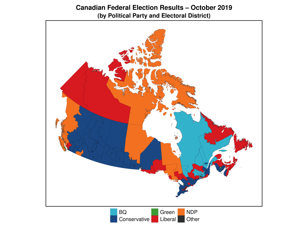
As I have noted in previous versions of this data visualization series, standard electoral-result area maps often obfuscate and mislead/misrepresent rather than clarify and illuminate. This is especially the case in electoral systems that are based on single-member electoral districts in which there is a single winner in every district (as known as ‘first-past-the-post’). Below you can see an example of a typical map used by the media (and others) to represent an electoral outcome. The map below is a representation of the results of the 2019 Canadian Federal Election, after which the incumbent Liberal Party (with Justin Trudeau as Prime Minister) was able to salvage a minority government (they had won a resounding majority government in the 2015 election).

There are two key guiding constitutional principles of representation regarding Canada’s lower house of parliament—the House of Commons: i) territorial representation, and ii) the principle of one citizen-one vote. As of the 2019 election these principles, combined with other elements of Canadian constitutionalism (like federalism) and the course of political history, have created the current situation in which the 338 federal electoral districts vary not only in land area, but also in population size, and often quite dramatically (for a concise treatment on this topic, click here).

Because a) “land doesn’t vote,” and b) we only know the winner of each electoral district (based on the colour) and not how much of the vote this candidate received) the map below misrepresents the relative political support of parties across the country. As of 2016, more than 2/3 of the Canadian population lived within 100 kilometres of the US border, a total land mass that represents only 4% of Canada’s total.

I’ve created a map that splits Canada in two—each colour represents 50% of the total Canadian population. You can see how geographically-concentrated Canada’s population really is.

The electoral ridings in red account for half of Canada’s population, while those in light grey account for the other half. Keep this in mind whenever you see traditional electoral maps of Canada’s elections.

## This is code for the first map above. This assumes you 
## have crated an sf object named can_sf, which has these 
## properties:

```
Simple feature collection with 6 features and 64 fields
Geometry type: MULTIPOLYGON
Dimension:     XY
Bounding box:  xmin: 7609465 ymin: 1890707 xmax: 9015737 ymax: 2986430
Projected CRS: PCS_Lambert_Conformal_Conic
```

library(ggplot2)
library(sf)
library(tidyverse)

gg.can <- ggplot(data = can_sf) +
  geom_sf(aes(fill = partywinner_2019), col="black", lwd=0.025) + 
  scale_fill_manual(values=c("#33B2CC","#1A4782","#3D9B35","#D71920","#F37021","#2B2D2F"),name ="Party (2019)") +
  labs(title = "Canadian Federal Election Results \u2013 October 2019",
       subtitle = "(by Political Party and Electoral District)") +
  theme_void() + 
  theme(legend.title=element_blank(),
        legend.text = element_text(size = 16),
        plot.title = element_text(hjust = 0.5, size=20, vjust=2, face="bold"),
        plot.subtitle = element_text(hjust=0.5, size=18, vjust=2, face="bold"),
        legend.position = "bottom",
        plot.margin = margin(0.5, 0.5, 0.5, 0.5, "cm"),
        legend.box.margin = margin(0,0,30,0),
        legend.key.size = unit(0.65, "cm"))

ggsave(filename="can_2019_all.png", plot=gg.can, height=10, width=13)

Here is the code for the 50/50 map above:

#### 50% population Map
gg.50 <- ggplot(data = can_sf) +
  geom_sf(aes(fill = Land.50.Pop.2016), col="black", lwd=0.035) + 
  scale_fill_manual(values=c("#d3d3d3", "red"),
        labels =c("Electoral Districts with combined 50% of Canada's Population",
                "Electoral Districts with combined other 50% of Canada's Population")) +
  labs(title = "Most of Canada's Land Mass in Uninhabited") +
  theme_void() + 
  theme(legend.title=element_blank(),
        legend.text = element_text(size = 11),
        plot.title = element_text(hjust = 0.5, size=16, vjust=2, face="bold"),
        legend.position = "bottom", #legend.spacing.x = unit(0, 'cm'),
        legend.direction = "vertical",
        plot.margin = margin(0.5, 0.5, 0.5, 0.5, "cm"),
        legend.box.margin = margin(0,0,0,0),
        legend.key.size = unit(0.5, "cm"))
#       panel.border = element_rect(colour = "black", fill=NA, size=1.5))

ggsave(filename="can_2019_50_pct_population.png", plot=gg.50, height=10, width=13)

Data Visualization #8–a Treemap Addendum

A quick addendum to my last post using treemaps to begin the new year. As a reminder, I drew a couple of treemaps that showed the distribution of votes across US counties during the 2016 Presidential Election(s). There are more than 3,200 counties in the USA, and the vast majority of them have low populations. In fact, under 200 counties (or less than 7%) contain more than half of the population. That means that the other 3,000 counties comprise about 50% of the population. In short,, the distribution of people (and, therefore, of voters) is highly skewed. In fact, here’s a bonus chart–a histogram of US counties by population.

As we can see, the vast majority of counties have small populations, while a few counties have very large populations, including Los Angeles County, in which almost 3.5 million persons voted. The counties with large populations are so few in number that we can’t even see them on the chart. A count of 1 on the chart (y-axis) is a vertical distance that isn’t even 1 pixel in size, so it doesn’t show up on the graph.

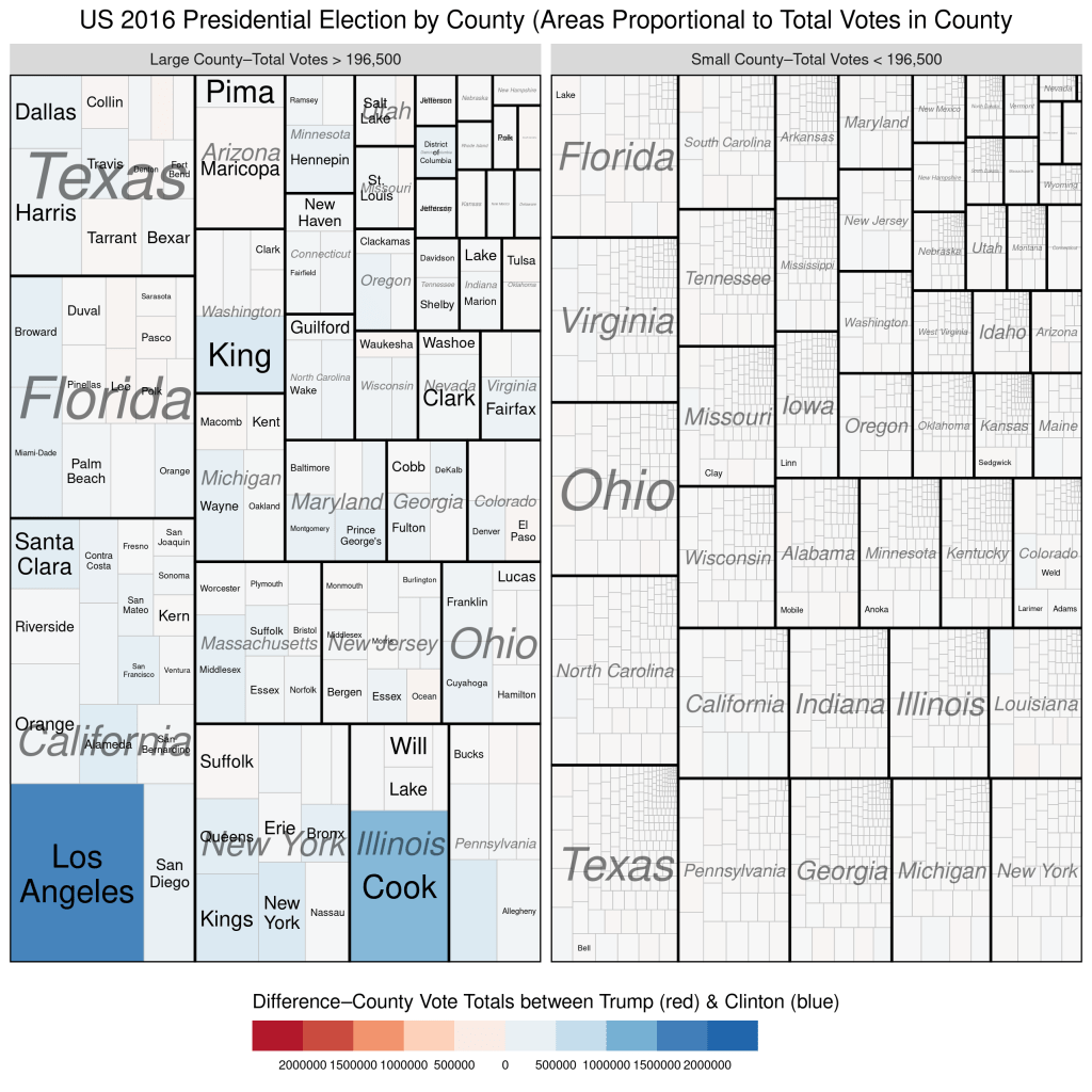
I’ve updated one of the treemaps from my previous post slightly to help reinforce the disparity in population size between the largest counties and the rest. In the treemap below, I’ve divided the counties into two groups–the largest counties versus the rest so that each group comprises 50% of the total votes cast. We see again, that a small number of counties (154 to be exact) combined to produce as many votes as the remaining ~3000 counties. Once again, we see that the counties won by Trump were, on average, so small that they there is not even a hint of red on the map. Here’s the treemap, with the R code below:

gg.tree.tot.facet <- ggplot(us_df_final_facet[us_df_final_facet$State.Name!="Hawaii",], 
        aes(area = totalvote, fill = vote_win_diff, label=NAME, subgroup=State.Name)) +
        geom_treemap() +
        geom_treemap_subgroup_border(colour="black", size=2) +
        geom_treemap_subgroup_text(place = "centre", grow=F, alpha = 0.5, colour =
                                           "black", fontface = "italic", min.size = 0) +
        geom_treemap_text(colour = "black", place = "center", reflow = T) +
        scale_fill_distiller(type = "div", palette=5, direction=1, guide="coloursteps", limits=c(-2000000,2000000), breaks=seq(-2000000,2000000, by=500000),
        labels=c("2000000","1500000","1000000","500000","0","500000","1000000","1500000","2000000")) +
        labs(title = "US 2016 Presidential Election by County (Areas Proportional to Total Votes in County",
             fill="Difference\u2013County Vote Totals between Trump (red) & Clinton (blue)") + 
        theme(legend.key.height = unit(0.6, 'cm'),
              legend.key.width = unit(2,"cm"),
              legend.text = element_text(size=7),
              plot.title = element_text(hjust = 0.5, size=14, vjust=1),
              legend.position = "bottom") +
        guides(fill = guide_coloursteps(title.position="top", title.hjust = 0.5),
               size = guide_legend(title.position="top", title.hjust = 0.5))  +
        facet_wrap( ~ countysize, scales = "free")

Data Visualization #7–Treemaps using US Counties and 2016 Presidential Vote

While we’re still waiting on the availability of official county-level results 2020 the 2020 US Presidential Elections*, I thought I’d create a treemap of the county-level results from the 2016 election. You may be thinking to yourself, “What is a treemap?”

Treemaps are ideal for displaying large amounts of hierarchically structured (tree-structured) data. The space in the visualization is split up into rectangles that are sized and ordered by a quantitative variable.

Link to Source

Treemaps, therefore, can help us visualize the relationships within our quantitative data in a unique, visually-pleasing, and meaningfully effective manner. Let’s see how with the example of the US 2016 Presidential Election.

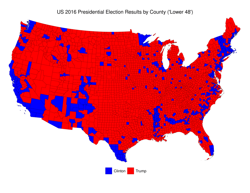
Here’s a picture of then newly-elected President Donald Trump looking at a map given to him by his advisers depicting the results of the 2016 election. This specific depiction of the results overstates the extent of the support across the USA for Trump in the 2016 election. As those in the know often say “land mass does not vote.” Indeed, if one were ignorant about US politics, and US political demography, looking at that map one would be most likely be perplexed were one told that the “blue” candidate actually won 3 million more votes than did the “red” candidate.

Here is my reproduction of these data\2013using publicly-available data from MIT Election Data and Science Lab, 2018, “County Presidential Election Returns 2000-2016”, https://doi.org/10.7910/DVN/VOQCHQ, Harvard Dataverse, V6, UNF:6:ZZe1xuZ5H2l4NUiSRcRf8Q== [fileUNF]. I’ve added the R-code at the end of this post.

We can see that the vast majority of counties are small, and that voters in these counties were more likely to have voted for Trump than for Clinton. Indeed, Clinton win fewer than 16% of all counties.

The problem with this map is that it essentially dichotomizes quantitative data into qualitative data. To be precise, the decision whether to colour a county blue or red is made simply on the basis of whether, of those who voted, more voted for Trump, or for Clinton. If a county voted 51-50 for Trump, it gets a red colour. If a county voted 1,000,000-100,000 for Clinton it gets coloured blue. And, to make things even more confusing, the total of red that each county receives is related ONLY to country land area, and doesn’t take account of the number of voters.

As is the case in many parts of the world today, the US is increasingly split demographically\u2013with those living in rural areas (and suburbs/exurbs) voting for the conservative parties (Republican) and those in the urban areas voting for liberal parties (Democratic). We see this clearly in the map above. The problem with US counties is that they are not uniform either in terms of their land area, or their population. There are apartment buildings in New York City and Los Angeles that have more residents than some counties.

We can use treemaps to more “accurately” depict electoral outcomes. By accurately, I mean that the visual representation of the data more closely reflects how many voted for each candidate (party).

The first example below represents the vote at the county level and describes two quantitative variables. The size of each rectangle represents the total number of voters in each county\u2013the larger the rectangle the greater the numbers of voters in that county. The second variable, which is mapped using the colour scale, represents the difference\u2013in raw vote totals between the two candidates. Reddish shades denote a county that was won by Trump, while bluish shades represent counties won by Clinton.

There are a couple of things to notice. First, the wide disparity in the total number of voters across the counties. Second, we see that most of the counties have shades that are only very lightly blue (or red) and look mostly white. This is because the range on the variable must be so expansive in order to include outliers like Los Angeles and Cook Counties. Thus, in the vast majority of US counties the raw vote total differences between Trump’s totals and Clinton’s totals are in the 1000s range. This is why Trump was able to win more than 84% of US counties and still lose the popular vote by more than 3 million.

Our next (and final) treemap is similar to the one above except that the scale for the colouring is not the raw vote difference between Trump and Clinton in each county, but the percentage-point differential in vote between the two candidates.

We see much more red and blue in this map because the scale is confined to 100% Trump win to 100% Clinton win. Notice the striking disparity in where the blue and red colours, respectively, are found. The reddish shades dominate in small-population counties (in the top-right corner of each state subgroup), while the bluish shades dominate in large-population counties (in the bottom-left corners of each state subgroup). Finally, the larger (greater population) counties tend be be much smaller geographically than the less-populous counties, which is why the map on Trump’s desk looks like it does.

gg.geom.uscounty <- ggplot(us_df_final_2163) +
        geom_sf(aes(fill = winner), col="black", lwd=0.1) + 
        scale_fill_manual(values=c("blue","red"), labels=c("Clinton","Trump"), breaks=c("Democrat","Republican")) + # breaks...to get rid of NA
        labs(title = "US 2016 Presidential Election Results by County ('Lower 48')") +
        theme_void() + 
        coord_sf(xlim = c(-1900000,2400000), ylim = c(-2050000, 625000)) +
        theme(legend.title=element_blank(),
              legend.text = element_text(size = 12),
              plot.title = element_text(hjust = 0.5, size=16, vjust=2),
              legend.position = "bottom",
              plot.margin = margin(0.5, 0.5, 0.5, 0.5, "cm"),
              legend.box.margin = margin(0,0,30,0),
              legend.key.size = unit(0.75, "cm"))

gg.geom.uscounty

R Code for treemaps: (this is vote the “total vote” variable. Replace that variable with a “percentage-vote” variable–with appropriate limits and breaks (-100,100) because you are now working with percentages).

gg.tree.tot <- ggplot(us_df_final, aes(area = totalvote, fill = vote_win_diff, label=NAME, subgroup=State.Name)) +
        geom_treemap() +
        geom_treemap_subgroup_border(colour="black", size=2) +
        geom_treemap_subgroup_text(place = "centre", grow=F, alpha = 0.5, colour =
                                           "black", fontface = "italic", min.size = 0) +
        geom_treemap_text(colour = "black", place = "center", reflow = T) +
        scale_fill_distiller(type = "div", palette=5, direction=1, guide="coloursteps", limits=c(-2000000,2000000), breaks=seq(-2000000,2000000, by=500000),
        labels=c("2000000","1500000","1000000","500000","0","500000","1000000","1500000","2000000")) +
        labs(title = "US 2016 Presidential Election by County (Areas Proportional to Total Votes in County",
             fill="Difference\u2013County Vote Totals between Trump (red) & Clinton (blue)") + 
        theme(legend.key.height = unit(0.75, 'cm'),
              legend.key.width = unit(2.35,"cm"),
              legend.text = element_text(size=8),
              plot.title = element_text(hjust = 0.5, size=14, vjust=1),
              legend.position = "bottom") +
        guides(fill = guide_coloursteps(title.position="top", title.hjust = 0.5),
               size = guide_legend(title.position="top", title.hjust = 0.5))    

* The electoral process that determines who becomes president of the United States is complicated. In effect, it is a series of elections that are run by individual states, and not a single federally-run election like it is in most presidential systems.

Data Visualization #6–US Counties are [essentially] Meaningless in Presidential Elections

The inspiration (so to speak) for this latest instalment of my Data Visualization series is a meme that I have been seeing spread across social media in the wake of the recent US Presidential Election. The meme, in essence, notes that numer of US counties (there are over 3000) that were “won” by the incumbent, Donald J. Trump. Indeed, it seems as though the challenger, Joe Biden, ironically won the most votes of any US Presidential candidate in US history while simultaneously having “won” the lowest percentage of counties (about 17%) of any winner of the Presidency ever.

Why did I place “won” in quotation marks? Two reasons: first, I am assuming that the authors of this meme suggest that Trump “won” these counties by having won (at least) a plurality of the vote in each. Which, I suppose, is true. The more important reason that I put “won” in quotation marks above is because US counties are effectively meaningless when it comes to determining who wins the US Presidency. They are only important insofar as receiving more votes than one’s opponent in any individual county helps increase the odds of winning what is important–a plurality of the vote in any individual state (or in Congressional Districts in the cases of Nebraska and Maine). Counties have no official weight when determining electoral college votes, and it doesn’t matter how many counties a candidate wins, as long as they reach at least 270 electoral votes. Counties in the USA vary in population from fewer than 100 (Kalawao County in Hawaii) to over 10,000,000 (Los Angeles County in California). So, discussing who “won” more counties is essentially meaningless.

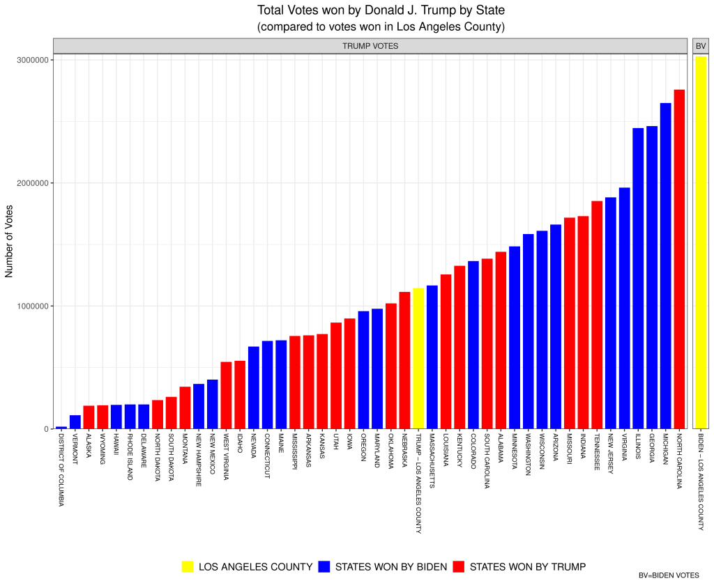
Here’s an example of how absurd referring to counties won becomes. The aforementioned Los Angeles County is a county that Joe Biden handily “won” in November, by a margin of 72.5% to 27.5% for Donald Trump. In short, Trump was walloped by Biden in LA County. Yet, when you compare Trump’s vote in LA County (about 1.15 million) to his total vote in all of the states (and DC) it might shock you to learn that Trump won more votes in LA County than he won in 25 individual states (and in DC). For example, Trump won more total votes in LA County (which, remember, he lost 72.5%-27.5%) than he won in the state of Oklahoma, where he won all 6 Electoral College votes. Moreover, Biden won more votes in LA County alone than Donald Trump won in each of all but three states–Florida, Texas, and Ohio. To be clear, for example, Biden won more total votes in LA County (which, alone, didn’t win him a single Electoral College vote) than Trump won in North Carolina (for which Trump won 15 Electoral College votes).

Here is a bar plot that I’ve created to visualize these data (click on the image to open a larger version). The yellow bar at the far-right represents the number of votes won by Biden in LA County (just over 3 million). The other yellow bar represents the votes won by Trump in LA Country (just over 1 million). Every other bar is the number of votes won by Trump in each of the states (and DC) listed below (Texas, Ohio, and Florida are missing because Trump won more votes in each of those states than Biden won in LA County). The red bars are states won by Trump, while the blue bars represent states won by Biden. Remember, each of the bars (except for the one on the far-right) represent the number of votes Donald Trump won in that state (and LA County).

Created by: Josip Dasovic

Data Visualization #4–Bar plots with widely-dispersed data

A common issue when trying to plot numerical data is the problem of outliers. When working with data the term outliers is often used in the statistical sense, referring to data certain data values that are “far way” from the rest of the data (in statistics, this usually means data values that are a number of standard deviations away from the rest of the data). This can be especially problematic when using common bar plots, especially when the minimum and maximum values are so far apart that it leads to difficulty representing all of the values visually.

For an example of this in real life, let’s have go back to our British Columbia provincial electoral map data. As I demonstrated in my first data visualization, area-based (rather than population-, or voter-based) maps are often misleading. The primary reason for this is that the electoral districts are not nearly the same size and don’t have the same numbers of residents. In British Columbia, a large province, (almost one million square kilometres in area) this is not a surprise, especially because of the manner in which the relatively small population (just over five million) is haphazardly-dispersed across the province.

We can easily calculate the population density of each of BC’s 87 provincial electoral districts, using data about district population size and calculating the area of each district from geographic we used to create the maps in the first data visualization post.

Here is a summary of the data (the variable is Pop.Den.km2):

(s1<-summary(bc_final_final$Pop.Den.km2))
     Min.   1st Qu.    Median      Mean   3rd Qu.      Max. 
    0.101     9.402   355.269  1587.483  2375.926 12616.797 

The “Min.” and “Max.” are the minimum, and maximum value, respectively, of the population density (persons per square kilometre) of BC’s 87 provincial electoral districts. We see a dramatic difference between the maximum and minimum values. In fact,

paste("The most densely-populated district is ", round(s1[6]/s1[1],0), "times as dense as the least densely-populated district.")

[1] "The most densely-populated district is 124551 times as dense as the least densely-populated district."

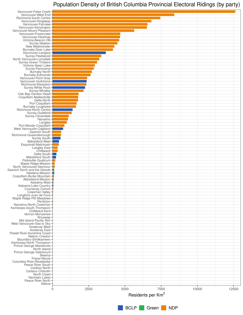
That is astounding, and if one were to simply plot these values on a bar chart, one would immediately recognize the difficulty with representing these data accurately. Let’s use a horizontal bar chart to demonstrate:

Here, we see that the larger numbers and so large, and the smaller numbers so comparatively small, that the lowest two dozen, or so, districts do not even seem to register. (When I first plotted this, I thought that I had made some sort of mistake and that the values at the bottom were missing. It turns out that the value represented by a single pixel was larger than the values of the districts at the bottom of the bar plot.)


This is obviously an issue–we don’t want to lose valuable information. There are alternative plots we could use, but we want to keep the information (political party) embodied in the various colours of the bar plot, so we’d like to find a bar plot solution. We’ll describe and assess two potential solutions in the next post in the series.

Data Visualization #3–Cartograms as an alternative to standard area-based electoral maps

In my first post of this series I explained at length why basic geographically-based electoral maps are not very good at conveying the phenomena of interest (see that post for more detail), and alluded to the increased use of political geographers, and political scientists, of alternative methods of “mapping” the required information that were more clear about the message(s) contained in the data.

Let’s examine this further using the map above. This map shows the results of the Canadian federal (national) election of October 2019.The respective proportions of total area “won” by each political party as depicted in the map above are not easily translated into either the relative vote share of the parties, or the relative number of seats won. Someone ignorant about Canadian federal politics would see a relatively similar total amount of red, blue, and orange, and assume that these parties had relatively equal support across the country. The sizes (land mass), and populations of, federal electoral districts in Canada vary drastically and, as a result, these maps are not a good gauge of voter support for political parties.

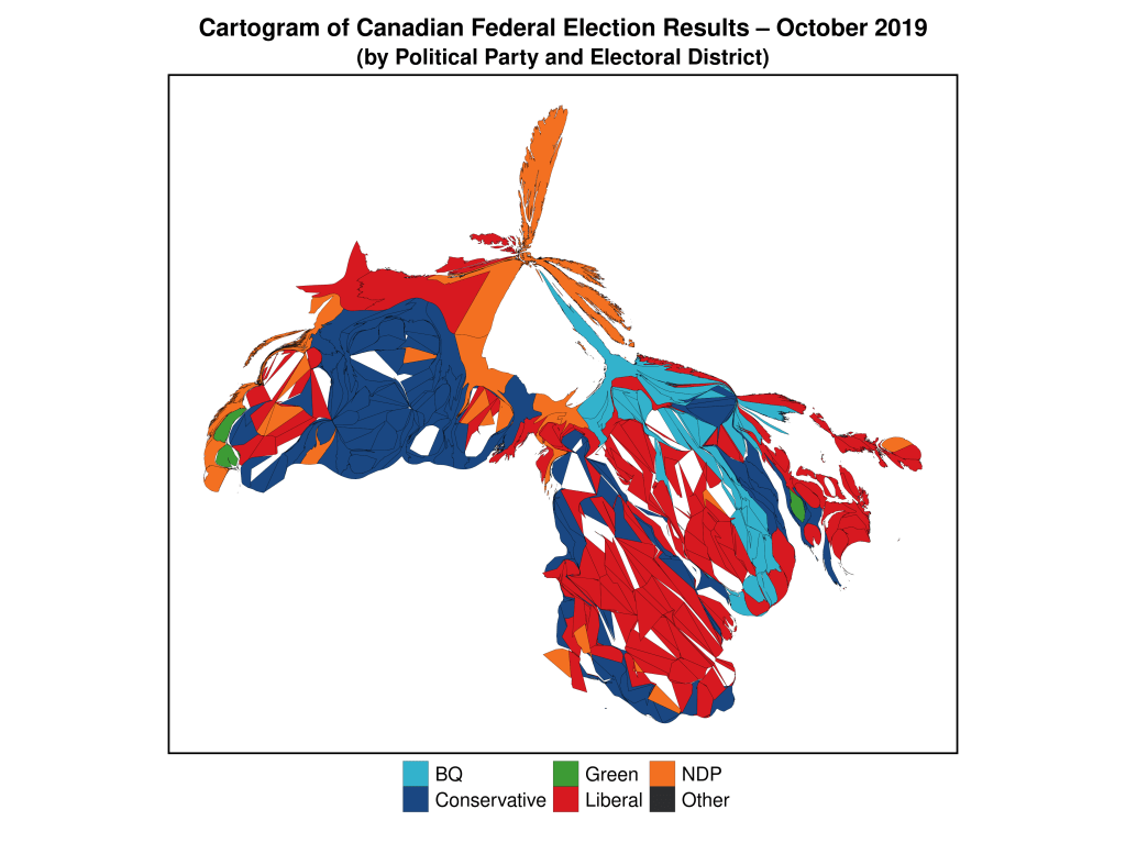
Since this problem is widespread political scientists, and political geographers, have attempted to find solutions to this problem. One increasingly-common approach has been to use what are called cartograms. Cartograms are maps in which the elements (in this case, electoral districts) are usually transformed in such as way as to maintain their connections to neighbours (contiguous cartograms), but to either increase or decrease the area of the specific electoral district in order to match it to a common variable. A variable often used in the transformation of electoral maps is population size. Thus, in a completed cartogram, the size of the electoral districts is not the actual land mass of the electoral district, but is proportional to the population of the electoral district (sometimes the number of voters, or the size of the electorate is used instead of population). It’s no surprise, then, that cartograms are also called “value-by-area” maps.

Cartograms are used by geographers and social scientists to depict a wide variety of phenomena. Here are some examples. The first one is a global cartogram for which the size of the area in each country is equivalent to total public health spending by that country. We can easily see that most of the world’s spending on public health occurs in the rich countries of the global north.

Here’s one more, depicting the global share of organic agriculture, by country.

Below, I have created a cartogram that has transformed the standard electoral map of the 2019 Canadian federal election into one in which the size of the electoral districts is mostly proportional to their populations. By “mostly” I mean that they’re not perfectly proportional, since the difference in sizes between the largest and smallest districts is so large the algorithm eventually stabilizes without creating completely equal-sized electoral districts.

This map more accurately conveys the nature of political partisan support (at least as it relates to the winning of electoral districts) across the country during the 2019 election, and provides visual evidence for the reality of an election in which the Liberal Party (red) won a plurality of the seats in the federal parliament (House of Commons). Because urban districts are much smaller than rural districts, the strength of Liberal Party support in Canada’s two largest cities–Toronto and Montreal–is obfuscated by the traditional area-based electoral map, but becomes evident in this cartogram.

The next map in this series will analyze another approach to geographically-based electoral maps–the hexagon map.

Here’s the R code for the cartogram above. Here, the original R-spatial data object–can_sf–is the base for the calculation of the cartogram data.

## Here is the code to generate the cartogram object:

library(cartogram)
can_carto_sf = cartogram_cont(can_sf, "Population_2016", itermax=50)

## Now, the map, using ggplot2
library(ggplot2)

gg.can.can.carto <- ggplot(data = can_carto_sf) +
  geom_sf(aes(fill = partywinner_2019), col="black", lwd=0.075) + 
  scale_fill_manual(values=c("#33B2CC","#1A4782","#3D9B35","#D71920","#F37021","#2B2D2F"),name ="Party (2019)") +
  labs(title = "Cartogram of Canadian Federal Election Results \u2013 October 2019",
       subtitle = "(by Political Party and Electoral District)") +
  theme_void() + 
  theme(legend.title=element_blank(),
        legend.text = element_text(size = 16),
        plot.title = element_text(hjust = 0.5, size=20, vjust=2, face="bold"),
        plot.subtitle = element_text(hjust=0.5, size=18, vjust=2, face="bold"),
        legend.position = "bottom",
        plot.margin = margin(0.5, 0.5, 0.5, 0.5, "cm"),
        legend.box.margin = margin(0,0,30,0),
        legend.key.size = unit(0.75, "cm"),
        panel.border = element_rect(colour = "black", fill=NA, size=1.5))

‘Controlling’ for confounding variables graphically

As we’ve learned (ad nauseum) basing causal claims on a simple bivariate relationship is fraught with potential roadblocks. Even though there may be a strong, and statistically significant, relationship between an independent and dependent variable, if we haven’t controlled for potentially confounding variables, we can not state with any measure of confidence that the putative relationship between the IV and DV is causal. We should always statistically control for any (and all) potentially confounding variables.

Additionally, it is often desirable to dig deeper into the data and find out if the units-of-analysis are fundamentally different on the basis of some other variable. Below you may find two plots–each of which shows the relationship between margin of victory and electoral turnout (by electoral district) for the 2017 British Columbia provincial election. The first graph plots a simple bivariate relationship, while the second plot breaks that initial relationship down by political party (which party won the electoral district). It could conceivably be the case that the relationship between turnout and margin of victory varies across the values of political party. That is, the relationship may hold in those electoral districts where party A won, but not hold in those in which party B won.

We can see here that there is little evidence to suggest a difference in the relationship based on which party won the electoral district. Can you think of another `third’ variable that may cause the relationship between turnout and margin of victory to be systematically different across different values of that variable? What about rural-versus-urban electoral districts?

Here are the plots:

You may not be registered to vote even though you think you are.

I read a somewhat troubling story this morning about Canadian citizens who have previously not only been registered to vote, but who have voted, and are no longer registered with Elections Canada. Here is an excerpt:

Delaney Ryan is a 23-year-old anthropology student at Simon Fraser University. Unlike many of her contemporaries, she voted in both the last provincial and federal elections. She meets all the criteria for voter registration, having her driver’s licence and maintaining the same address since voting in those elections.

She can’t understand why, then, this time, she wasn’t registered on the voters list.

“I had heard rumours about people not being registered, and a friend’s Facebook page had postings on it of other people finding out they were suddenly no longer registered. A lot of these people seemed to be in the same demographic as me. So I went online (to the Elections Canada website) and checked, and I wasn’t on it, either.

“So I had to reapply for registration.”

So, go to the Elections Canada website and verify that you are registered to vote this October 19.