Data Visualization #17—Land Doesn’t Vote, Citizens Do

As I have noted in previous versions of this data visualization series, standard electoral-result area maps often obfuscate and mislead/misrepresent rather than clarify and illuminate. This is especially the case in electoral systems that are based on single-member electoral districts in which there is a single winner in every district (as known as ‘first-past-the-post’). Below you can see an example of a typical map used by the media (and others) to represent an electoral outcome. The map below is a representation of the results of the 2019 Canadian Federal Election, after which the incumbent Liberal Party (with Justin Trudeau as Prime Minister) was able to salvage a minority government (they had won a resounding majority government in the 2015 election).

There are two key guiding constitutional principles of representation regarding Canada’s lower house of parliament—the House of Commons: i) territorial representation, and ii) the principle of one citizen-one vote. As of the 2019 election these principles, combined with other elements of Canadian constitutionalism (like federalism) and the course of political history, have created the current situation in which the 338 federal electoral districts vary not only in land area, but also in population size, and often quite dramatically (for a concise treatment on this topic, click here).

Because a) “land doesn’t vote,” and b) we only know the winner of each electoral district (based on the colour) and not how much of the vote this candidate received) the map below misrepresents the relative political support of parties across the country. As of 2016, more than 2/3 of the Canadian population lived within 100 kilometres of the US border, a total land mass that represents only 4% of Canada’s total.

I’ve created a map that splits Canada in two—each colour represents 50% of the total Canadian population. You can see how geographically-concentrated Canada’s population really is.

The electoral ridings in red account for half of Canada’s population, while those in light grey account for the other half. Keep this in mind whenever you see traditional electoral maps of Canada’s elections.

## This is code for the first map above. This assumes you 
## have crated an sf object named can_sf, which has these 
## properties:

```
Simple feature collection with 6 features and 64 fields
Geometry type: MULTIPOLYGON
Dimension:     XY
Bounding box:  xmin: 7609465 ymin: 1890707 xmax: 9015737 ymax: 2986430
Projected CRS: PCS_Lambert_Conformal_Conic
```

library(ggplot2)
library(sf)
library(tidyverse)

gg.can <- ggplot(data = can_sf) +
  geom_sf(aes(fill = partywinner_2019), col="black", lwd=0.025) + 
  scale_fill_manual(values=c("#33B2CC","#1A4782","#3D9B35","#D71920","#F37021","#2B2D2F"),name ="Party (2019)") +
  labs(title = "Canadian Federal Election Results \u2013 October 2019",
       subtitle = "(by Political Party and Electoral District)") +
  theme_void() + 
  theme(legend.title=element_blank(),
        legend.text = element_text(size = 16),
        plot.title = element_text(hjust = 0.5, size=20, vjust=2, face="bold"),
        plot.subtitle = element_text(hjust=0.5, size=18, vjust=2, face="bold"),
        legend.position = "bottom",
        plot.margin = margin(0.5, 0.5, 0.5, 0.5, "cm"),
        legend.box.margin = margin(0,0,30,0),
        legend.key.size = unit(0.65, "cm"))

ggsave(filename="can_2019_all.png", plot=gg.can, height=10, width=13)

Here is the code for the 50/50 map above:

#### 50% population Map
gg.50 <- ggplot(data = can_sf) +
  geom_sf(aes(fill = Land.50.Pop.2016), col="black", lwd=0.035) + 
  scale_fill_manual(values=c("#d3d3d3", "red"),
        labels =c("Electoral Districts with combined 50% of Canada's Population",
                "Electoral Districts with combined other 50% of Canada's Population")) +
  labs(title = "Most of Canada's Land Mass in Uninhabited") +
  theme_void() + 
  theme(legend.title=element_blank(),
        legend.text = element_text(size = 11),
        plot.title = element_text(hjust = 0.5, size=16, vjust=2, face="bold"),
        legend.position = "bottom", #legend.spacing.x = unit(0, 'cm'),
        legend.direction = "vertical",
        plot.margin = margin(0.5, 0.5, 0.5, 0.5, "cm"),
        legend.box.margin = margin(0,0,0,0),
        legend.key.size = unit(0.5, "cm"))
#       panel.border = element_rect(colour = "black", fill=NA, size=1.5))

ggsave(filename="can_2019_50_pct_population.png", plot=gg.50, height=10, width=13)

Data Visualization #16—Canadian Federal Equalization Payments per capita

My most recent post in this series analyzed data related to the federal equalization program in Canada using a lollipop plot made with ggplot2 in R. The data that I chose to visualize—annual nominal dollar receipts by province—give the reader the impression that over the last five-plus decades the province of Quebec (QC) is the main recipient (by far) of these federal transfer funds. While this may be true, the plot also misrepresents the nature of these financial flows from the federal government to the provinces. The data does not take into account the wide variation in populations amongst the 10 provinces. For example, Prince Edward Island (PEI) as of 2019 has a population of about 156,000 residents, while Quebec has a population of approximately 8.5 million, or about 55 times as much as PEI. That is to say a better way of representing the provincial receipt of equalization funds is to calculate the annual per capita (i.e., for every resident) value, rather than a provincial total.

For the lollipop chart below, I’ve not only calculated an annual per-capita measure of the amount of money received by province, I’ve also controlled for inflation, understanding that a dollar in 1960 was worth a lot more (and could be used to buy many more resources) in 1960 than today. Using Canadian GDP deflator data compiled by the St. Louis Federal Reserve, I’ve created plotting variable—annual real per-capita federal equalization receipts by province, with a base year of 2014. Here, we see that the message of the plot is no longer Quebec’s dominance but a story in which Canadians (regardless of where they live) are treated relatively equally. Of course, every year, Canadian in some provinces receive no equalization receipts.

Here’s the plot, and the R code below it:

Source: https://open.canada.ca/data/en/dataset/4eee1558-45b7-4484-9336-e692897d393f
require(ggplot2)
require(gganimate) 

gg.anim.lol3 <- ggplot(eq.pop.df[eq.pop.df$Year!="2019-20",], aes(x=province, y=real.value.per.cap, label=real.value.per.cap.amt)) + 
  geom_point(stat='identity', size=14, aes(col=as.factor(zero.dummy))) +  #, fill="white"
  scale_color_manual(name="zero.dummy", 
                     #      labels = c("Above", "Below"), 
                     values = c("0"="#000000", "1"="red")) + 
  labs(title="Per Capita Federal Equalization Entitlements (by Province): {closest_state}",
       subtitle="(Real $ CAD—2014 Base Year)",
       x=" ", y="$ CAD (Real—2014 Base Year)") +
  geom_segment(aes(y = 0, 
                   x = province, 
                   yend = real.value.per.cap, 
                   xend = province), 
               color = "red",
               size=1.5) +
  scale_y_continuous(breaks=seq(0,3000,500)) +
  theme(legend.position="none",
        plot.title =element_text(hjust = 0.5, size=23),
        plot.subtitle =element_text(hjust = 0.5, size=19),
        axis.title.x = element_text(size = 16),
        axis.title.y = element_text(size = 16),
        axis.text.y =element_text(size = 14),
        axis.text.x=element_text(vjust=0.5,size=16, colour="black")) +
  geom_text(color="white", size=4) +
  transition_states(
    Year,
    transition_length = 1,
    state_length = 9
  ) +
  enter_fade() +
  exit_fade()

animate(gg.anim.lol3, nframes = 610, fps = 10, width=800, height=680, renderer=gifski_renderer("equal_real_per_cap_lollipop.gif"))  

Data Visualization #15—Canadian Federal Equalization Payments over time using an animated lollipop graph

There is likely no federal-provincial political issue that stokes more anger amongst Albertans (and is so misunderstood) as equalization payments (entitlements) from the Canadian federal to the country’s 10 provinces. Although some form of equalization has always been a part of the federal government’s policy arsenal, the current equalization program was initiated in the late 1950s, with the goal of providing, or at least helping achieve an equal playing field across the country in terms of basic levels of public services. As Professor Trevor Tombe notes:

Regardless of where you live, we are committed (indeed, constitutionally committed) to ensure everyone has access to “reasonably comparable levels of public services at reasonably comparable levels of taxation.”

Finances of the Nation, Trevor Tombe

For more information about the equalization program read Tombe’s article and links he provides to other information. The most basic misunderstanding of the program is that while some provinces receive payments from the federal government (the ‘have-nots’) the other, more prosperous, provinces (the ‘haves’) are the source of these payments. You often hear the phrase “Alberta sends X $billion to Quebec every year!” That’s not the case. The funds are generated and distributed from federal revenues (mostly income tax) and disbursed from this same fund of resources. The ‘have’ provinces don’t “send money” to other provinces. The federal government collects tax revenue from all individuals and if a province has a higher proportion of high-earning workers than another, it will generally receive less back in money from the federal government than its workers send to Ottawa. (To reiterate, read Tombe for more about the particulars.)

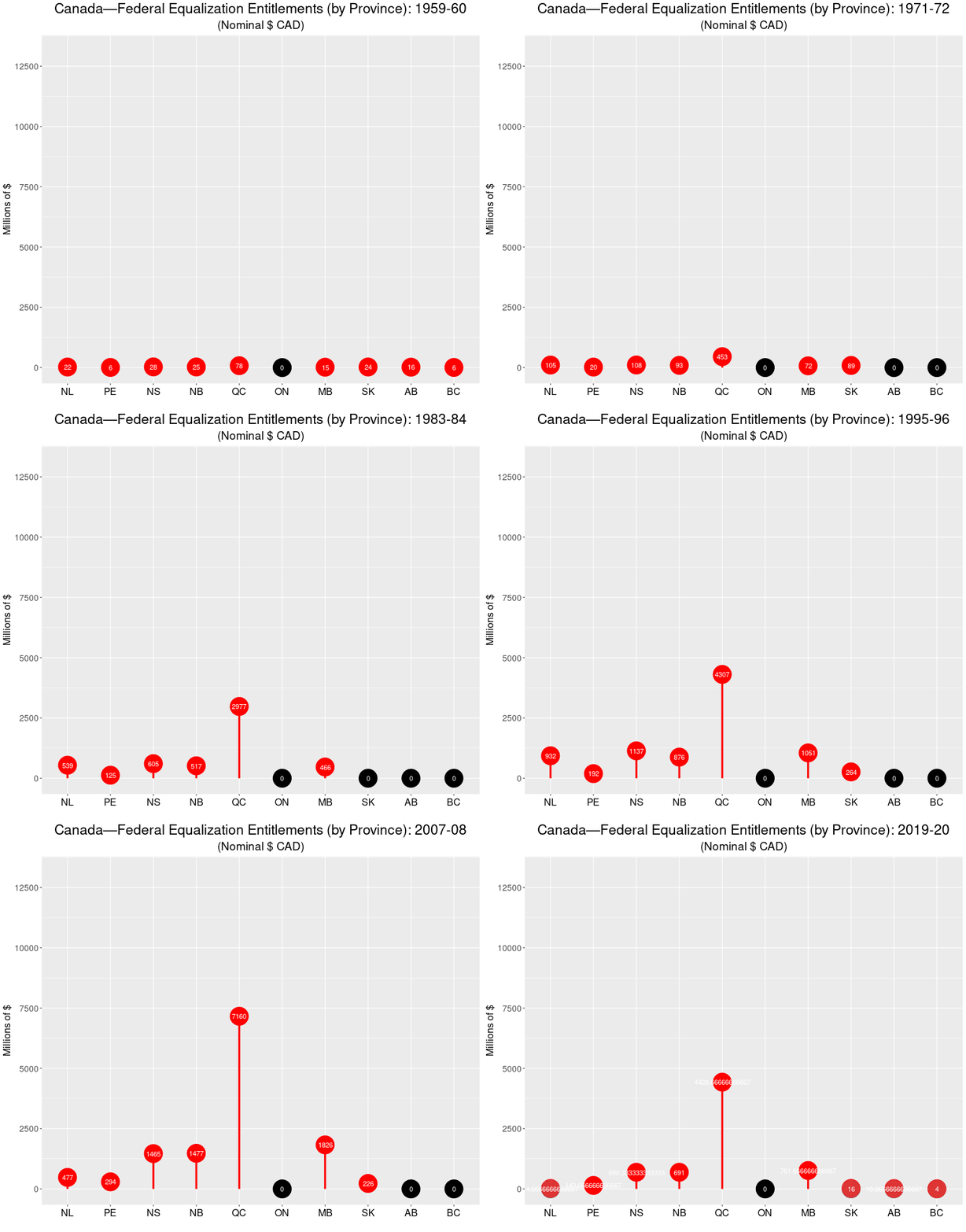
Using data provided by the Government of Canada, I have decided to show the federal equalization outlays over time using what is called a lollipop chart. I could have used a bar chart, but I like the way the lollipop chart looks. Here’s the chart and the R code below:

Created by Josip Dasović

The data source is here: https://open.canada.ca/data/en/dataset/4eee1558-45b7-4484-9336-e692897d393f, and I am using the table called Equalization Entitlements.

N.B.: The original data, for some reason, had Alberta abbreviated as AL, so I had to edit the my final data frame and the gif.

## You'll need these two libraries
require(ggplot2)
require(gganimate)

gg.anim.lol1 <- ggplot(melt.eq.df, aes(x=variable, y=value, label=amount)) + 
  geom_point(stat='identity', size=14, aes(col=as.factor(zero.dummy))) +  #, fill="white"
  scale_color_manual(name="zero.dummy", 
                     values = c("0"="#000000", "1"="red")) + 
  labs(title="Canada—Federal Equalization Entitlements (by Province): {closest_state}",
       x=" ", y="Millions of nominal $ (CAD)") +
  geom_segment(aes(y = 0, 
                   x = variable, 
                   yend = value, 
                   xend = variable), 
               color = "red",
               size=1.5) +
  scale_y_continuous(breaks=seq(0,15000,2500)) +
  theme(legend.position="none",
        plot.title =element_text(hjust = 0.5, size=23),
        axis.title.x = element_text(size = 16),
        axis.title.y = element_text(size = 16),
        axis.text.y =element_text(size = 14),
        axis.text.x=element_text(vjust=0.5,size=16, colour="black")) +
  geom_text(color="white", size=4) +
    transition_states(
  Year,
  transition_length = 2,
  state_length = 8
) +
  enter_fade() +
  exit_fade()

animate(gg.anim.lol1, nframes = 630, fps = 10, width=800, height=680, renderer=gifski_renderer("equal.lollipop.gif"))  

Data Visualization #14—Using python to create animated charts

In my previous post I noted that I would provide python code for the chart that is in the post. The chart was created using R statistical software, and the code for the python version can be found at the end of this post.

I find python a bit less intuitive than R but that’s most likely because I’ve been using R for a very long time and python for less long. There are reasons, I suppose, to favour one over the other, but for statistical analysis and data analysis I don’t necessarily see an advantage of one over the other. That being said, it is my sense that R does a better job of standardizing across various operating systems, which can be very helpful when you are a Linux user, as am I.

import numpy as np
import matplotlib.pyplot as plt
import networkx as nx
from matplotlib.animation import FuncAnimation 
plt.style.use('ggplot') # this is to make the plot look like an R ggplot

# a roulette array
roulette = np.append(np.array([0, 0]),np.arange(1, 37))
spins1000 = np.array(np.random.choice(roulette, size=(1000)))

# Define a cumulative mean function
def cum_mean(arr):
    cum_sum = np.cumsum(arr)
    return cum_sum / (np.arange(1, cum_sum.shape[0] + 1))     # as far as I can tell, matplotlib doesn't have a cumulative mean function; so I created one.


fig = plt.figure()
ax1 = fig.add_subplot(2, 1, 2)
ax2 = fig.add_subplot(2, 1, 1)
fig.tight_layout(pad=3.0)
fig.suptitle('Short-term Randomness versus Long-term Predictability', fontsize=14) 
ax2.set_xlabel('$n^th$ spin of roulette wheel')
ax2.set_ylabel('Value of $n^{th}$ spin')
ax2.set_xlim(0, 1000)
ax2.set_ylim(0, 37)

ax1.set_xlabel('$n^{th}$ spin of the roulette wheel')
ax1.set_ylabel('Cumulative mean of n spins')
ax1.set_xlim(0, 1000)
ax1.set_ylim(0, 37)

line, = ax1.plot([], [], lw=1.5)
scat, = ax2.plot([], [], 'o', markersize=2)

def init():
    line.set_data([], [])
    scat.set_data([], [])
    return line, scat,

def animate(i):
    x = np.linspace(0, 250, 250)
    y1 = cum_mean(spins1000)
    y2 = spins1000
    line.set_data(x[:i], y1[:i])
    scat.set_data(x[:i], y2[:i])
    return line, scat,

anim = FuncAnimation(fig, animate, init_func=init, frames=1000, interval=10, blit=True, save_count=1000)

plt.show()

anim.save('roullete_python.mp4') # saving as .mp4 because python creates massive gif files.

Data Visualization #13—Roulette and Temperature with R code

In the most recent post in my data visualization series I made an analogy between climate, weather and the spins of a roulette wheel that demonstrated that short-term randomness does not mean we can’t make accurate long-term predictions.

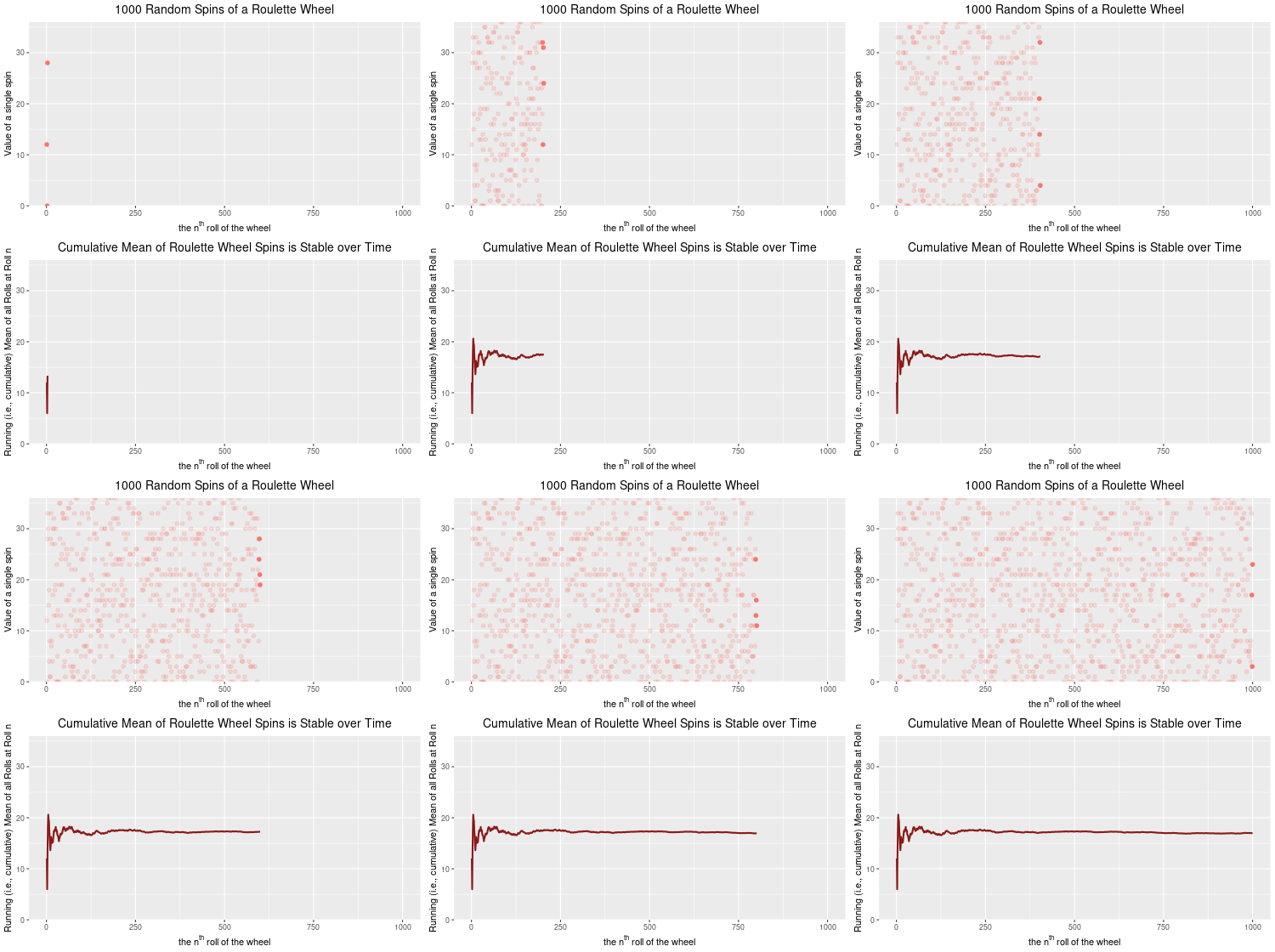
Towards the end of the post I appended an animation of 1000 random spins of a roulette wheel. In that post, I plotted the 1000 individual outcomes of these random spins of the roulette wheel. I chose to show only one outcome at a time as the animation cycled through all 1000 spins. In this post, I wanted to show you how to keep all of the outcomes from disappearing. Rather than having the value of each spin appear, and then disappear, I will change the code slightly to have every spin’s outcome stay on the plot, but faded so that the focus remains on the next spin value. Here’s what I mean.:

Created by Josip Dasović

Here is the R code for the image above:

## These are the packages needed to draw, and animate, the plots.
library(ggplot2)
library(gganimate)
library(dplyr)  # needed for cummean function

## Set up a data frame for the 1000 random spins of the roulette wheel

mywheel <-c(rep(0,2),1:36)  # a vector with the 38 wheel values
wheel.df<-data.frame("x"=1:1000,"y"=sample(mywheel,1000,rep=T))

## Plot, then animate the result of 1000 random spins of the wheel

## the code to plot
gg.roul.1000.point<- ggplot(wheel.df,aes(x, y, colour = "firebrick4")) + 
  geom_point(show.legend = FALSE, size=2) +
  theme_gray() + 
  labs(title = "1000 Random Spins of a Roulette Wheel", 
       x = expression("the"~n^th~"roll of the wheel"), 
       y = 'Value of a single spin') +
  theme(plot.title = element_text(hjust = 0.5, size = 14, color = "black")) +
  scale_y_continuous(expand = c(0, 0)) +
  transition_time(wheel.df$x) +
  shadow_mark(past = T, future=F, alpha=0.2)

## the code to animate
gg.roul.anim.point <- animate(gg.roul.1000.point, nframes=500, fps=25, width=500, height=280, renderer=gifski_renderer("gg_roulette_1000.gif"))  
 
## No plot and animate a line chart that depicts the cumulative mean from spin 1 to spin 1000.

gg.roul.1000.line <- ggplot(wheel.df, aes(x, y = cummean(y))) +
  geom_line(show.legend = FALSE, size=1, colour="firebrick4") +
  theme_gray() +
  ggtitle("Cumulative Mean of Roulette Wheel Spins is Stable over Time") +
  theme(plot.title = element_text(hjust = 0.5, size = 14, color = "black")) +
  labs(x = expression("the"~n^th~"roll of the wheel"), 
       y = 'Running (i.e., cumulative) Mean of all Rolls at Roll n') +
  scale_y_continuous(expand=c(0,0), limits=c(0,36)) +
  transition_reveal(wheel.df$x) +
  ease_aes('linear') 

gg.roul.anim.line <- animate(gg.roul.1000.line, nframes=500, fps=25, width=500, height=280, renderer=gifski_renderer("cummean_roulette_1000.gif"))  

## Now combine the plots into one figure, using the magick library

library(magick)

a_mgif <- image_read(gg.roul.anim.point)
b_mgif <- image_read(gg.roul.anim.line)

roul_gif <- image_append(c(a_mgif[1], b_mgif[1]),stack=TRUE)
for(i in 2:500){
  combined <- image_append(c(a_mgif[i], b_mgif[i]),stack=TRUE)
  roul_gif <- c(roul_gif, combined)
}

## Save the final file as a .gif file

image_write(roul_gif, "roulette_stacked_point_line_500.gif")

Stay tuned for a Python version of this chart.

Data Visualization # 12—Using Roulette to Deconstruct the ‘Climate is not the Weather’ response to climate “deniers”

If you are at all familiar with the politics and communication surrounding the global warming issue you’ll almost certainly have come across one of the most popular talking points among those who dismiss (“deny”) contemporary anthropogenic (human-caused) climate change (I’ll call them “climate deniers” henceforth). The claim goes something like this:

“If scientists can’t predict the weather a week from now, how in the world can climate scientists predict what the ‘weather’ [sic!] is going to be like 10, 20, or 50 years from now?”

Notably, the statement does possess a prima facie (i.e., “commonsensical”) claim to plausibility–most people would agree that it is easier (other things being equal) to make predictions about things are closer in time to the present than things that happen well into the future. We have a fairly good idea of the chances that the Vancouver Canucks will win at least half of their games for the remainder of the month of March 2021. We have much less knowledge of how likely the Canucks will be to win at least half their games in February 2022, February 2025, or February 2040.

Notwithstanding the preceding, the problem with this denialist argument is that it relies on a fundamental misunderstanding of the difference between climate and weather. Here is an extended excerpt from the US NOAA:

We hear about weather and climate all of the time. Most of us check the local weather forecast to plan our days. And climate change is certainly a “hot” topic in the news. There is, however, still a lot of confusion over the difference between the two.

Think about it this way: Climate is what you expect, weather is what you get.

Weather is what you see outside on any particular day. So, for example, it may be 75° degrees and sunny or it could be 20° degrees with heavy snow. That’s the weather.

Climate is the average of that weather. For example, you can expect snow in the Northeast [USA] in January or for it to be hot and humid in the Southeast [USA] in July. This is climate. The climate record also includes extreme values such as record high temperatures or record amounts of rainfall. If you’ve ever heard your local weather person say “today we hit a record high for this day,” she is talking about climate records.

So when we are talking about climate change, we are talking about changes in long-term averages of daily weather. In most places, weather can change from minute-to-minute, hour-to-hour, day-to-day, and season-to-season. Climate, however, is the average of weather over time and space.

The important message to take from this is that while the weather can be very unpredictable, even at time-horizons of only hours, or minutes, the climate (long-term averages of weather) is remarkably stable over time (assuming the absence of important exogenous events like major volcanic eruptions, for example).

Although weather forecasting has become more accurate over time with the advance of meteorological science, there is still a massive amount of randomness that affects weather models. The difference between a major snowstorm, or clear blue skies with sun, could literally be a slight difference in air pressure, or wind direction/speed, etc. But, once these daily, or hourly, deviations from the expected are averaged out over the course of a year, the global mean annual temperature is remarkably stable from year-to-year. And it is an unprecedentedly rapid increase in mean annual global temperatures over the last 250 years or so that is the source of climate scientists’ claims that the earth’s temperature is rising and, indeed, is currently higher than at any point since the beginning of human civilization some 10,000 years ago.

Although the temperature at any point and place on earth in a typical year can vary from as high as the mid-50s degrees Celsius to as low as the -80s degrees Celsius (a range of some 130 degrees Celsius) the difference in the global mean annual temperature between 2018 and 2019 was only 0.14 degrees Celsius. That incorporates all of the polar vortexes, droughts, etc., over the course of a year. That is remarkably stable. And it’s not a surprise that global mean annual temperatures tend to be stable, given the nature of the earth’s energy system, and the concept of earth’s energy budget.

In the same way that earth’s mean annual temperatures tend to be very stable (accompanied by dramatic inter-temporal and inter-spatial variation), we can see that the collective result of many repeated spins of a roulette wheel is analogously stable (with similarly dramatic between-spin variation).

A roulette wheel has 38 numbered slots–36 of which are split evenly between red slots and black slots–numbered from 1 through 36–and (in North America) two green slots which are numbered 0, and 00. It is impossible to determine with any level of accuracy the precise number that will turn up on any given spin of the roulette wheel. But, we know that for a standard North American roulette wheel, over time the number of black slots that turn up will be equal to the number of red slots that turn up, with the green slots turning up about 1/9 as often as either red or black. Thus, while we have no way of knowing exactly what the next spin of the roulette wheel will be (which is a good thing for the casino’s owners), we can accurately predict the “mean outcome” of thousands of spins, and get quite close to the actual results (which is also a good thing for the casino owners and the reason that they continue to offer the game to their clients).

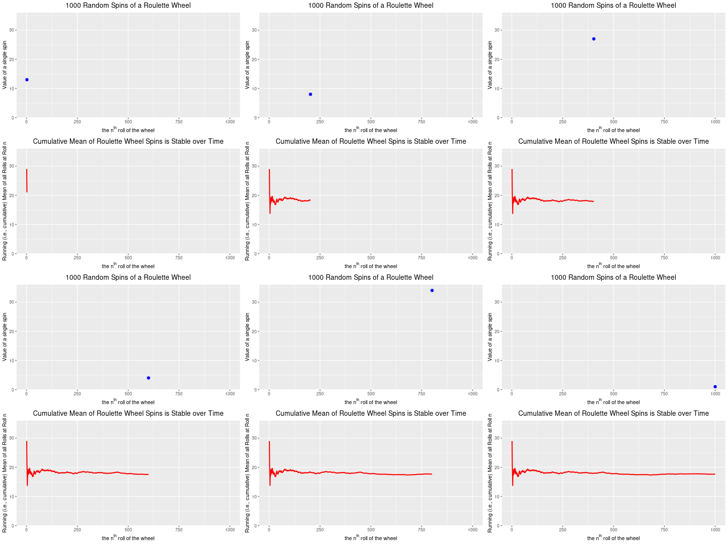
Below are two plots–the upper plot is an animated plot of each of 1000 simulated random spins of a roulette wheel. We can see that the value of each of the individual spins varies considerably–from a low of 0 to a high of 36. It is impossible to predict what the value of the next spin will be.

The lower plot, on the other hand is an animated plot, the line of which represents the cumulative (i.e. “running”) mean of 1000 random spins of a roulette wheel. We see that for the first few random rolls of the roulette wheel the cumulative mean is relatively unstable, but as the number of rolls increases the cumulative mean eventually settles down to a value that is very close to the ‘expected value’ (on a North Amercian roulette wheel) of 17.526. The expected value* is simply the sum of all of the individual values 0,0, 1 through 36 divided by the total number of slots, which is 38. Over time, as we spin and spin the roulette wheel, the values from spin-to-spin may be dramatically different. Over time, though, the mean value of these spins will converge on the expected value of 17.526. From the chart below, we see that this is the case.

Created by Josip Dasović

Completing the analogy to weather (and climate) prediction, on any given spin our ability to predict what the next spin of the roulette wheel will be is very low. [The analogy isn’t perfect because we are a bit more confident in our weather predictions given that the process is not completely random–it will be more likely to be cold and to snow in the winter, for example.] But, over time, we can predict with a high degree of accuracy that the mean of all spins will be very close to 17.526. So, our inability to predict short-term events accurately does not mean that we are not able to predict long-term events accurately. We can, and we do. In roulette, and for the climate as well.

TLDR: Just because a science can’t predict something short-term does not mean that it isn’t a science. Google quantum physics and randomness and you’ll understand what Einstein was referring to when he quipped that “God does not play dice.” Maybe she’s a roulette player instead?

  • Note: This is not the same as the expected dollar value of a bet given that casinos generate pay-off matrixes that are advantageous to themselves.

Data Visualization #11—X-rays

If you sit down for a minute and think about it, an x-ray is the culmination of a data generating, and visualization, process. What we see on the screen is a representation (or a model) of the body part being x-rayed. Over a month ago (hence the disruption to my blogging routine) I unexpectedly had knee replacement surgery (yay for cancellation lists!). Here is an x-ray of my new right knee (airport scanners, here I come!):

The parts showing very white are new and will hopefully allow me to hike and bike pain-free from this point on. It’s been a painful, but ultimately productive, healing and rehabilitation process and I’ll be continuing my data visualization challenge beginning next week. See you soon!